Creating a Loan Amortization Schedule in Google Sheets

Does Google Sheets Have a Loan Amortization Schedule?

One of the biggest fears of small business or people just starting out is getting a loan.  Filling out the paperwork for the bank or car dealership is scary.  Come with us and take some control by learning how to make and use a loan amortization schedule to understand and keep track of your loan like we do.  Let’s get Started!

We like to hike.  So, as we walk you through this schedule in Google Sheets I hope you don’t mind us sharing some views of the Grand Canyon like this view from Bright Angel Trail. We’ll tackle the loan amortization schedule by working through a series of questions.  Watch the whole video to uncover how valuable this worksheet will be to your business and personal finances.  Our first question really starts the process of understanding loans:

What is the PMT Function in Google Sheets?

The PMT function in Google Sheets or PMT is used to calculate the payment for a loan based on a constant interest rate, the total number of payments, and the loan amount. It's particularly useful when you want to determine the monthly payment on a car loan or any other type of loan with a fixed interest rate.  So, the main inputs you need to know are the amount of the loan, the interest rate of the loan, and the loan term.  The loan term is how many months or years the loan will be outstanding which is also how long you will be making payments.  So, let’s work through a loan that is for $150,000 and has an interest rate of 7% with a 30 year term.  Almost all loans have these three things and all basic loans will work this way.  To learn the monthly payment for this loan type in =pmt open parentheses(b12 which is the interest rate/12 months, the months of the loan or 360, and the present value, or the loan amount close parenthesis). I also added a - sign after the equals as the PMT function returns a negative amount without the minus sign.  Here you will see the monthly payment will be $997.95.  

Now that we understand the payment function and how to find out what your monthly payment will be we should understand the loan further by building an amortization schedule.  

Let’s start with the month column and answer

How Do You Insert Sequential Numbers in Google Sheets?

We are going to have a row for each month in our loan amortization schedule in Google Sheets.   So the first column will be titled month.  Under that I am going to type in 1,2,3,4 in subsequent rows.  Now to insert sequential numbers I can use my mouse and highlight a7:a10 and then left click on the cell anchor and while holding the click dragging the mouse down the column.  When I’ve reached a good spot release the click and the cells will populate with a sequential list of numbers.  Here you can see me go to 40.  You can also do this with dates and other numbers in a series.  But, there is another way to insert a list of numbers.  I can use the formula =+the cell above, in this case a46 + 1.  Now in a47 you can see the number 41.  Now I can copy and paste that formula as far down the sheet as I would like.  For our loan amortization schedule we want to get to 360 months or 30 years * 12 months. Now to get back to the top let’s use the shortcut keys CTRL+Home

Google Sheets builds on a foundation of basic skills.  In order to build this loan amortization schedule we need to know the efficient ways to insert a sequential list like the two we just shared with you.  Join (above) or Subscribe (YouTube) today to take your Google Sheets education to the next level.  By subscribing the next time you search for anything Google Sheets our videos will come up at the top of your search results.  

Ok, This schedule is still looking unfinished. So, while we hike South Kaibab trail let’s continue with

How Can I Track Lan Payments in Google Sheets?

Now that we have the series of months listed in Column A we need to build out the column titles for the information we need to track your loan payments in Google Sheets.  The information we need to track loan payments are the Beginning loan amount, the payment, the interest amount, and the principal amount and the ending loan amount.  Interest is the amount you pay the bank each month for borrowing money from them.  But, the principal amount is the amount of money the loan was reduced by with the payment.  As you make payments these columns will help you understand where you’ve been with the loan, where you are going, and as important where you are.  As we continue with the design you’ll see how it all comes together.

How Do I Create a Loan Amortization Schedule in Google Sheets?

Here is where the schedule starts to come together.  We have our Month column filled out but have to work on the rest.  The Beginning amount column will be the loan amount outstanding before each payment for that month.  Here in cell b7 we will type in =b1 to capture the amount financed.  In cell b7 we will type in =$b$4, the strings are also known as dollar signs to capture the monthly payment amount calculated above and we will use the $ as we will copy that cell later.  The interest formula in cell d7 will be =b7*(b2/12) and we will use relative cell referencing or strings to lock B2 . The result is $875.00.  The principal will be the payment amount less the interest amount so type in cell e7 =c7-d7 which is $122.95.  The ending amount is the ending amount of the loan after the payment so we will type in f7 =b7-e7

How Can I Tell How My Loan Payment Changes Over the Life of a Loan?

Now that we have the first payment detailed we can work on month 2 and the rest of the schedule.  The beginning loan amount for month 2 will be the ending loan amount from month 1.  So, in cell b8 type in =f7.  The payment doesn’t change so you will want to copy cell c7 to c8 or type in cell c8 =$b$4.  Again the relative cell referencing so we always pick B4 if we copy and paste this cell.  But, the interest amount will be calculated so in cell d8 type in =b8*($B$2/12).  The 12 is to take the annual interest of 7% and get the rate to a monthly amount because most loans require monthly payments.  The principal amount will again be the payment less interest or type in cell e8 =c8-d8.  The ending amount will be the Beginning Amount less the Principal or type in cell f8 =b8-e8.  Now row 8 can be copied down the schedule.  So, copy B8 - F8 and paste down every row until you get to the 360th month row or row 366. 

So, now you can see each month detailed in the Google Sheet.  A little tip here is to go to cell b8 and use shortcut keys CTRL-SHIFT right arrow, then CTRL+C to copy.  Then go to the month column and CTRL+ down arrow to get to the last month, then in cell b366 CTRL+Shift+ up arrow and CTRL+V to paste.  These shortcut keys make copy and paste go a lot faster.  So now you can see each month detailed in the Google Sheet.

How Do You Remove the Dollar Sign in Google Sheets?  

I like to format my Google Sheets schedules to only have dollar signs on the first row and the total rows if any.  Over the years I’ve learned it's a traditional accounting format that I like.  So, to remove the dollar signs from the rest of the rows I am going to highlight the cells to format.  Then click the 123 number format button and click the number format.  Here you will see all of the dollar signs removed.  

Now that the schedule is almost done we’ll start reading and understanding the schedule next.  But, if you want a copy of this schedule click here!

What Does a Loan Payment Tracker in Google Sheets do?

So, now that we have the loan amortization schedule built in Google sheets let’s analyze what it can do.  You can see in this example in column D that the loan starts off with monthly payments mainly going to interest.  In column E only $122.95 is going to principal.  Long duration loans like this will provide a lower payment but a lot of interest expense.  Let’s add a couple of columns to track interest and principal.  In cell G6 title the column Accumulated interest.  In cell g7 type in =d7 and in cell g8 type  in =d8+g7.  Now if you copy g8 down the column you will notice the interest expense on this $150,000 loan is almost $210,000.  But, type in H6 Accumulated Principal and format the cell to center, wrap text, and add a bottom border.  In cell h7 type in =e7.  In cell h8 type in =e8+h7.  Copy cell h8 down the column to learn how much principal is paid off.  At the bottom you will see the loan of $150,000 is paid off proving the schedule works as designed.    

But what if we change the dollar amount of the loan to $100,000?  We’ll see the interest expense reduces to $139,508 with a monthly payment of $665.30.  But how about we change the term of the loan to 20 years.  Here you will see the interest is only $86,000 but the payment increased to $775.30 per month.  But, if I change the interest rate to 6.5% we’ll see the payment reduces to $745.57 and the interest reduces to just under $79,000.  If we wanted to make this more of a car payment let’s change the amount to $30,000 with a 5 year term.   At 5 years the payment is about $587 with $5,219.07 in interest paid to the bank.

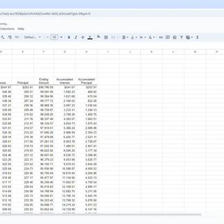
But what if we make extra principal payments to reduce the loan faster?  Here we will type in 1500 in month 20 cell c26 and 1200 in cell c28 and 1000 in cell c30.  Everything calculates and the loan is paid off 5 months earlier.  

If you want to take your Google Sheets skills to the next level read one of these posts next!